\(\renewcommand\AA{\unicode{x212B}}\)
Table of Contents
This custom interface will integrate several tasks related to engineering diffraction. In its current state it provides functionality for creating and loading calibration files and focusing ENGINX run files.
Functionality for performing single peak fitting on focused run files is currently in progress.
This interface is under active development.
The location of files saved by the GUI during processing will be shown in the mantid messages log.
Note: The locations are shown at “Notice” level, so may not appear if the messages log is on the incorrect setting.
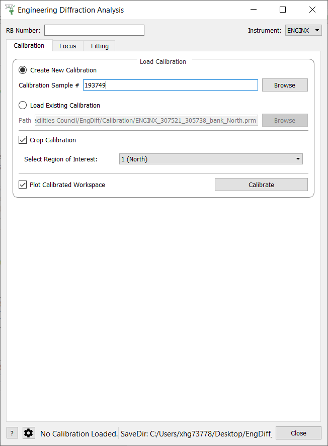
This tab currently provides a graphical interface to create new calibrations and visualise them. It also allows for the loading of GSAS parameter files (.prm) created by the calibration process to load a previously created calibration into the interface.
When loading an existing calibration, the fields for creating a new calibration will be automatically filled, allowing the recreation of the workspaces and plots generated by creating a new calibration.
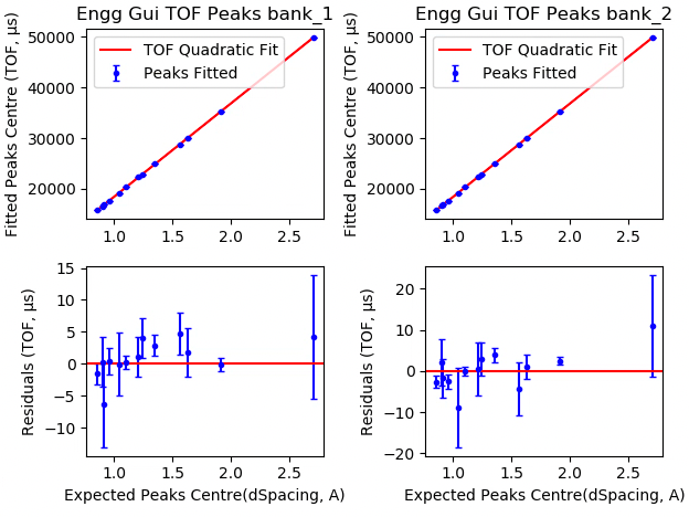
The “Plot Output” check-box will plot the ceria peaks for new calibrations, one of each plot for each of the detector banks selected.
Creating a new calibration file generates instrument parameter files for the selected region of interest. If both banks are selected then two additional .prm files are created - one for each individual bank. The calibration files are written to the directory:
<CHOSEN_OUTPUT_DIRECTORY>/Calibration/
If an RB number has been specified the files will also be saved to a user directory in the base directory:
<CHOSEN_OUTPUT_DIRECTORY>/User/<RB_NUMBER>/Calibration/
The interface also provides the ability to restrict a new calibration to a particular region of interest: one of the two banks onn ENGIN-X, a custom .cal file or a custom list of spectra.


This tab allows for the focusing of data files - summing up spectra in a given region of interest. To do this a new or existing calibration must be created or loaded (see above) and a vanadium run must also be supplied for normalisation.
The data will be focused over the region of interest selected in the calibration tab. Files can be selected by providing run numbers or selecting the files manually using the browse button.
Ticking the “Plot Focused Workspace” checkbox will create a plot of the focused workspace when the algorithm is complete (if both banks have been focused there will be a plot for each bank).
Clicking the focus button will begin the focusing algorithm for the selected run files. The button and plotting checkbox will be disabled until the fitting algorithm is complete.
The focused output files are saved in NeXus, GSS, and TOPAS format. All of these files are saved to:
<CHOSEN_OUTPUT_DIRECTORY>/Focus/
If an RB number has been specified the files will also be saved to a user directory:
<CHOSEN_OUTPUT_DIRECTORY>/User/<RB_NUMBER>/Focus/


This tab will allow for plotting and peak fitting of focused run files.
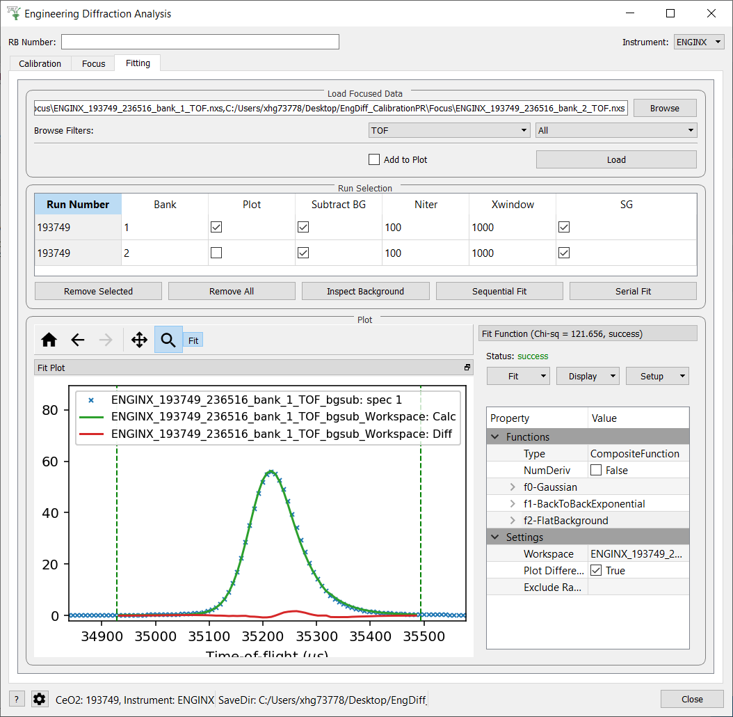
Focused run files can be loaded from the file system into mantid from the interface. The interface will keep track of all the workspaces that it has created from these files. When a focused run is loaded, the proton charge weighted average (and standard deviation) of the log values set in the settings options are calculated and stored in a grouped workspace accessible in the main mantid window.
Loaded workspaces can be plotted in the interface and the mantid fitting capability can be accessed from the ‘Fit’ button on the plot toolbar. This allows for the user to select peaks of any supported type (the default is BackToBackExponential) by right-clicking on the plot. The initial parameters can be varied interactively by dragging sliders (vertical lines on the plot). After a successful fit the best-fit model is stored as a setup in the fit browser (Setup > Custom Setup) with the name of the workspace fitted. Selecting this loads the function and the parameters and the curve can be inspected by doing Display > Plot Guess.
The output from the fit is stored in a group of workspaces that contains a matrix workspace of the fit value and error for each parameter in the model. If there is more than one of the same function, the parameters are stored in the same workspace with different x-values. For example, if there were two Gaussian peaks then there would be a workspace for each parameter of the Gaussian (i.e. Height, PeakCentre, Sigma) each of which will have two columns corresponding to each peak. Each workspace has a spectra per run loaded (each row in the table of the UI fitting tab). In general different models/functions could be fitted to each run, so when there is a parameter that does not exist for a run (or that run has not yet been fitted), the Y and E fields in the relevant row are filled with NaNs. The group of fit workspaces also contains a table workspace that stores the model string that can be copied into the fit browser (Setup > Manage Setup > Load From String).
The workspaces can be fitted sequentially (sorted by the average of a chosen log in the settings) or serially (fitted with the same initial parameters). If a valid model is present in the fit browser then the Sequential Fit and Serial Fit buttons (below the table in the UI) will be enabled - it is not necessary to run an initial fit.
The user may want to fix or constrain certain model parameters, which can be done in the usual way in the fit browser. The sequential fit will populate the fit tables as above and store the model in the Custom Setups.

Categories: Interfaces | Diffraction